A Complete Guide to Machine Learning

This guide is divided into 6 main categories:

How Neural Nets Work
Machine Learning Models
Math of Machine Learning
Python for Machine Learning
Understanding Data Normalization
Understanding Gradient Descent and Backpropagation

How Neural Nets Work

A neural net is simply a network of neurons.

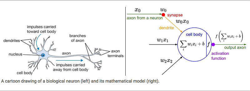
Inspired by a neurons in the human brain; a single layer neural net is called a perceptron. A perceptron performs a simple linear calculation for binary classification.

A perceptron is a type of a feed forward neural net which only does a forward pass. A forward pass is when an output is generated from an input via a simple linear function.

In neural nets if we stack these perceptrons upon each other a mesh of perceptrons are formed. This mesh of perceptron is known as a multi-layer perceptron (MLP). We use MLP for multi-class classification problems. MLP use backpropogation to solve problems.

Example of a feed forward neural net

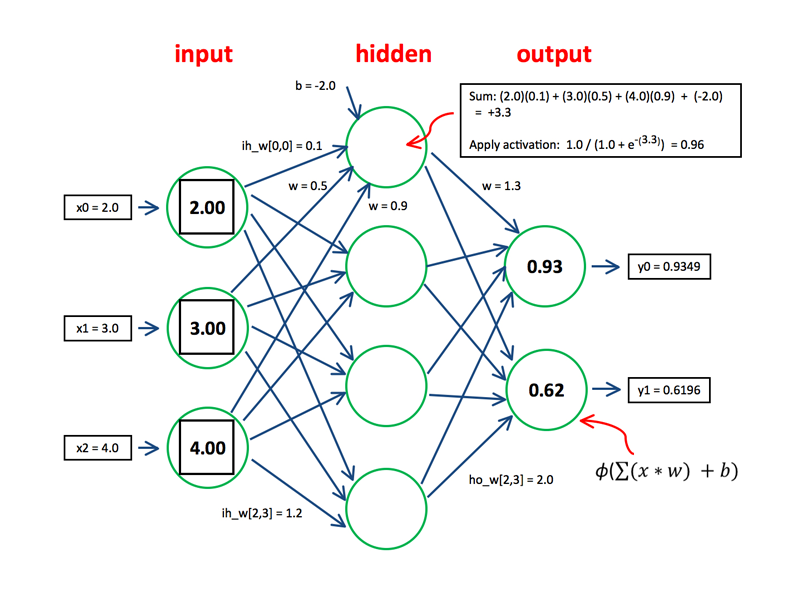
Diagram solution

The input of the perceptron is a matrix of numbers which repreesent a binary class.

If we look at the first neuron x0 we see the input is multiplied by a particular weight.

We multiply each input with the assigned weight.

x = input, w = weight 

input + weight = E

(x0 * w0) + (x1 * w1) + (x2 * w2)

(2.0 * 0.1) + (3.0 * 0.5) + (4.0 * 0.9) = 5.3

After we multiply each input by the weight we are left with the value of E which is 5.3

b = bias, Y = b + E

E + bias = Y

5.3 + (-2.0) =  3.3

After that we simply add the bias which is -2 and we are left with the value of Y which is 3.3

This value (Y) is then passed through an activation function.

Why do we use an activation function?

Our Y value has no bounds it could be infinite. Hence, we need to pass it through an activation function to give it a restricted finite value so our neural net can make a prediction.

A = activation function 

A = sigmoid(Y)

In this case we use a sigmoid non-linear function.

Y is then passed through the activation function of your choosing (sigmoid, tanh, relu) which converts our Y of 3.3 into A of 0.96.

Now we can make a binary classification depending on the threshold of the the value we calculated.

Machine Learning Models

The world of artificial intelligence is an interesting place to be a part of these days. Due to the cheap and ubiquitous access to computing power in form of CPUs, GPUs and TPUs has made it easier for researchers and organizations to harness the power of predictive modelling and analysis.

In order to understand the nature of the problem, I typically ask the following questions:

What is the nature, size and quality of your data?
What hardware do you have to run the model?
What are you trying to find? (if you don’t know what you’re looking for then yer dun goofed!)

But in order to understand when to use a model from the plethora of options we need to know the types of problems we can solve and in which category your problem falls under.

Machine Learning falls under the following 5 categories:

Supervised Learning
Unsupervised Learning
Semi-supervised Learning
Reinforcement Learning
Recommendation Engine

In Supervised Learning we have labelled data. If we have categorical data we can use Classification algorithms if the data is continuous we are better off with Regression. Anomalies fall under anomaly detection.

In Unsupervised Learning our data is non-labelled and we need to make sense of this data by putting them in clusters i.e. Clustering or reduce the dimensions to find the meaningful ones using Association rules.

Semi-Supervised Learning contains a mix of labelled and unlabeled data.

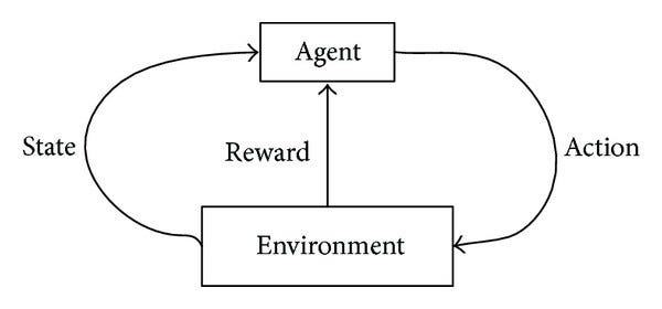
In Reinforcement Learning we could have both types of data. The model takes an action to maximize the reward function in an environment.

Reinforcement learning can be better explained by reward feedback or the reinforcement signal.

Recommendation Engine is an approach where the algorithm finds patterns in historical data to give accurate and meaningful recommendations. Due to its complexity I like to give Recommendation Engine its own category!

Popular Machine Learning Algorithms

Linear Regression: Estimating coefficients of a model to predict an output with a given input.
Logistic Regression: Estimates coefficients like LR but uses maximum-
likelihood estimation.
Decision Trees: Uses greedy algorithm on the training data to estimate splits in the tree.
Naive Bayes: A probabilistic model used for both binary and multi-class classification.
k-Nearest Neighbors: KNN model generates predictions by calculating similarity between train and test data.
Learning Vector Quantization: LVQ model is an artificial neural net (ANN) algorithm that makes predictions like KNN but learns from the training set.
Support Vector Machines: SVM model uses different types of classifiers (maximal-margin, soft margin) and converts the data into a kernel (linear, polynomial, radial) to made predictions.
Random Forests: RF combines predictions from multiple variance models using bagging techniques (also known as Bagged Random Forests).
Boosting: Boosting (AdaBoost or XGBoost)adds weak learners to correct
classification errors to make accurate predictions.

Math of Machine Learning

Before you begin your journey in Machine Learning (ML) and Deep Learning (DL) you should at least know the basic math behind what you will be doing. Although you can still dive right into algorithms and implementation of code you will have a severe handicap against your data science peers.

Everyone is at some level daunted by math. But once you understand its real world application to data science, it becomes inherently more fun and useful.

The mathematics for machine learning can be divided into 3 main categories:

Linear Algebra
Calculus
Statistics and Probability

Linear Algebra

Question: Why study linear algebra?

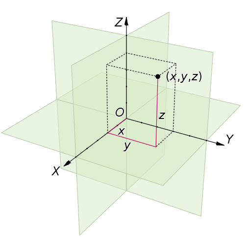
Answer: By using linear algebra we can solve “linear equations”. Linear equations can be represented in the forms of matrices. A matrix in machine learning is how we represent our features. We can represent data in 0 dimension (scalar), 1 dimension (vector), 2 dimensions (matrix) and n-dimensions (tensor).

A simple linear equation is y = wx + b

where;

y = y-axis, x = x-axis, w = slope, b = y-intercept

However in machine learning;

y = prediction, b= bias, w = weight of feature, x = feature

Question: Why do we need to study logarithms?

Answer: In machine learning you will have to deal with big data (millions of rows and countless features). Logs help us express large numbers efficiently. And most importantly they will help us solve exponential equations like sigmoid (know as activation function in deep learning). After studying linear algebra you will learn how to solve linear equations, represent your data in dimensions and understand logarithms.

Tutorials

For beginners (high school math only): Start with this tutorial.

For intermediate (college level math only): Start with this tutorial.

Fun fact: The world algebra comes from Muḥammad ibn Mūsā al-Khwārizmī (ca. 750–ca. 850) who used it to solve linear and quadratic equations.

Calculus

Calculus tell us how things change. In machine learning we make predictions and calculus helps us make them. In calculus you will need to study derivatives, partial derivatives, gradients and chain rules.

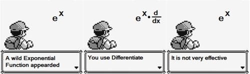
Question: Why study derivatives?

Answer: A derivative simply shows the rate of change; the amount by which a function is changing at one given point. In machine learning we will need to find the minimum point in our function where the prediction we make is the optimal. Derivatives help us do that. Partial derivatives are a very similar to derivatives as well.

Question: Why study gradients?

Answer: A gradient is simply the slope of a graph. In machine learning we use a powerful optimization technique called gradient descent known as backpropagation in deep learning. Gradient descent is simple terms help us to find the local minima which reduces our prediction error.

Great visual tutorial on backpropagation can be found here.

Tutorials

For beginners (high school math only): Start with this tutorial

For intermediate (college level math only): Start with this tutorial

Fun fact: Isaac Newton and Gottfried Leibniz independently discovered calculus in the mid-17th century. Both died disputing who came up with it first.

Statistic and Probability

In machine learning in any type of problem either regression on classification your algorithm will compute a probability from the features. In order to interpret what the accuracy means we will need to study stats and probability.

Question: Why study statistics?

Answer: Stats is a powerful tool for data scientists; you will learn how to analyze data and visualize data. Stats is mainly used in the data preprocessing stage.

Types of variables:

Discrete variables: Variables which can be counted (e.g. number of lions)

Continuous variables: Variables which can be measured (e.g. height,weight)

Question: Why use summary statistics?

Answer: So we can quickly summarize the most important points of our data. Summary statistics includes; central tendency, mean, median, mode, standard deviation, skewness, kurtosis, range, interquartile range and charts (histogram, scatter plot, pie chart, line chart etc.)

Central Tendency: Describes the central tendency of a data via mean, median, mode

Mean: Sum of all observations/ number of observations

Median: The middle observation

Mode: The most common observation

Range: All respective observations in a group

Interquartile Range: Range of observations largest to smallest

Variance: Squared difference of observation from mean / number of observation

Standard deviation: Square root of variance.

Question: Why is Standard deviaton so important?

Answer: We use standard deviation to measure how our data is distributed. The greater the spread the greater the standard deviation.

Hypothesis testing: In data science, you always start with a hypothesis. Your goal is to reject the null hypothesis.

Types of Error 1&2:

Type 2 errors are more dangerous than Type 1 errors

Skewness: Measure the lack of symmetry in our data. Symeetrical data will have perfect symmetry on both sides.

Kurtosis: Measure whether the data are heavy-tailed or light-tailed relative to a normal distribution.

Normal distribution: Values plotted on a graph which are bell shaped. Great primer on normal distribution and its importance can be found here.

If data looks normal use = z, t, ANOVA, Chi, F test

If data is skewed use = Chi, F test

Question: Why use Probability?

Answer: Probability simply means chance of an event happening. We use the range of 0 – 100% to describe the chance of a particular event happening. 0 being no chance, 100 being an absolute.

Conditional Probability: Simply means the chance of an A event happening, if event B has already happened.

Tutorials

For beginners (high school math only): Start with this tutorial.

For intermediate (college level math only): Start with this tutorial.

Fun Fact: Al-Kindi developed the first code breaking algorithm based on frequency analysis.

Python for Machine Learning

I understand. You’re tired. You just want to start programming in Python so you can start doing cool projects.

Well the good thing is that Python is a very intuitive language. Its actually the preferred language for data scientists (sorry R!). So I have assembled a quick guide for you to learn Python in a matter of minutes!

Python falls in the class of object-oriented languages. It has many great libraries for data science including pandas, numpy, sci-kit learn, matplotlib etc.

This aim of this guide is for you to get up to speed with Python so you hit the ground running.

We will be using Python 3 (the latest iteration)

For this lesson we wont be installing and IDE on our computer. We will use an online IDE to compile our code. For that please click HERE

First Program

#Open the IDE
#The first program for any programming language is “Hello World”

print ("Hello World")

# Execute

Hello World

Base Types

# Integer 
# int 5 56 69 0

int = 5 56 69 0

# Float
# float 9.45 0.55

float = 9.45 0.55

# Boolean
# bool True False

# String
# str "One" "Ahsan"

str = "One" , "Ahsan"

Variables in Python

# Declaring a variable
# Whenever you use = you are assigning a value to some variable
#For example we use an integer

a = 1
print (a)

# Execute

1

# Re-assigning string to the same variable

a = "Ahsan"
print (a)

# Execute

Ahsan

#Concatenate Variables a & b

a = "Ahsan"
b = 1989

print (a+b)

# Execute

Traceback (most recent call last):
  File "python", line 4, in <module>
  TypeError: must be str, not int

# We got an error becasue we cannot add an integer & a string
# Hence we will convert integer to a string
# Use str function

print (a+str(b))

# Execute

Ahsan1989

# If we want to add a space between an integer and string
# Use " "

print (a+" "+str(b))

# Execute

Ahsan 1989

#Deleting a variable
# Delete b

del b

print (a+" "+str(b))

# Execute

Traceback (most recent call last):
  File "python", line 8, in <module>
  NameError: name 'b' is not defined

# b gets deleted hence the above NameError

Transforming Variables

#Accessing value in strings

a = "Ahsan"

print(a[0])

# Execute

A

# 0 is the first position in the variable
# Same can be done with multiple variables

a = "Ahsan"
b = "Will be teaching you python"
c = "How cool is that?"

print(a[0:5],b[0:20],c[0:8])

# Execute

Ahsan Will be teaching you How cool

Lists

# A list is a container type for storing different base types in Python

# also called an array

# List can be changed

list1 = [1, 2, 4]
list2 = ["Ahsan", "Anis", 1989]

# Accessing different values in a list

print(list1[1])

# Execute

2

print(list2[0:1])

# Execute

['Ahsan']

Tuples

# Tuples are like lists but are immutable meaning they cannot be changed

tuple1 = (1, 2, 4)
tuple2 = ("Ahsan", "Anis", 1989)

print(tuple2[0:1])

# Execute

('Ahsan',)

Dictionary

# Dictionary is an immutable data type such as strings, numbers, or tuples

dict = {'Name': 'Ahsan', 'Age': 28, 'Position': 'Data Scientist'}

print (dict['Name'], dict['Age'], dict['Position'])

# Execute

Ahsan 28 Data Scientist

# Can also be written like this

dict = {'Name': 'Ahsan', 'Age': 28, 'Position': 'Data Scientist'}

print ("dict['Name']: ", dict['Name'])

print ("dict['Age']: ", dict['Age'])

print("dict['Position']:", dict['Position'])

# Execute

dict['Name']:  Ahsan
dict['Age']:  28
dict['Position']: Data Scientist

Arrays

# An array is a 1 dimensional data structure also known as a scalar

arr = [100, 200, 300, 400, 500]

print (arr[1:4])

# Execute

[200, 300, 400]

Matrix

# A  A matrix is a 2 dimensional data structure

matrix = [['Ahsan',8,8,8,8,8],
         ['Anis',9,9,9,9,9],
         ['Data',0,0,0,0,0],
         ['Scientist',1,1,1,1,1]]

print (matrix)

# Execute

[['Ahsan', 8, 8, 8, 8, 8], ['Anis', 9, 9, 9, 9, 9], ['Data', 0, 0, 0, 0, 0], ['Scientist', 1, 1, 1, 1, 1]]

Arithmetic Operators

# Addition

a =  100
b = 10

print (a+b)

# Execute

110

# Subtraction a-b = 90
# Multiplication  a * b = 1000
# Division a / b = 10
# Modulus a % b = 0 , b % a = 10
# Exponent a**b = 100000000000000000000

If statement

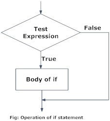
# If statetemnt is a boolean expression followed by one or more statements
# Boolean statement are either True or False

a = 100
if a > = 10:
     print ("Thats a big number")

# Execute

Thats a big number

If…Else statement

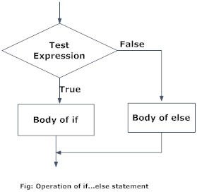
#If statement runs like usual, Else statement run if the first statement is False

a = 9
if a >= 10:
     print ("Thats a big number")
else:
    print ("Not a big number")

# Execute

Not a big number

Elif statement

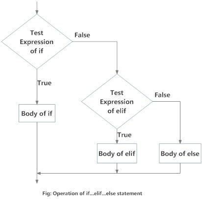
# Elif statement is a statement which you put after if statement

a = 1
if a > 0:
     print ("Thats a big number")
elif a == 0:
    print ("Not a big number")
else:
    print ("Put another number")

# Execute

Thats a big number

a = 0
if a > 0:
     print ("Thats a big number")
elif a == 0:
    print ("Not a big number")
else:
    print ("Put another number")

# Execute

Not a big number

a = -2
if a > 0:
     print ("Thats a big number")
elif a == 0:
    print ("Not a big number")
else:
    print ("Put another number")

# Execute

Put another number

Nested if statements

# An if, else, elif statement within an if, else, elif statement is called a nested if statement 

num = float(input("Enter a number: "))
if num >= 0:
    if num == 0:
        print("Zero")
    else:
        print("Positive number")
else:
    print("Negative number")

For Loop

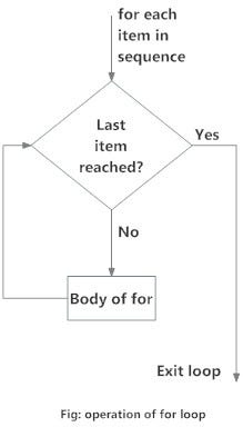
# a for loop executes till the last statement is reached

numbers = [1, 2, 2, 8, 4]

sum = 0

for val in numbers:
 sum = sum+val

print("The sum is", sum)

# Execute

('The sum is', 17)

For loop with else

# Exactly like for loop, just that the else statement is printed at the end

numbers = [1, 2, 3, 4, 5 , 6, 7, 8, 9, 10]

for i in numbers:
    print(i)
else:
    print("All numbers printed.")

# Execute

1
2
3
4
5
6
7
8
9
10
All numbers printed.

While loop

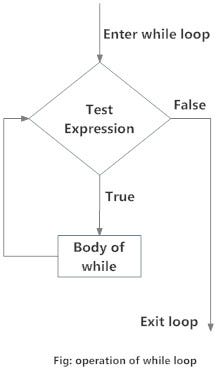
# a while loop iterates the statement as long as the statement is True

number = 0
while (number <= 10):
   print 'The count is:', number
   number = number + 1

print "All numbers printed"

# Execute

The count is: 0
The count is: 1
The count is: 2
The count is: 3
The count is: 4
The count is: 5
The count is: 6
The count is: 7
The count is: 8
The count is: 9
The count is: 10
All numbers printed

While loop with else

# Same as while loop, else statement is executed when logic is false

counter = 0

while counter <= 10:
    print("loop")
    counter = counter + 1
else:
    print("end loop")

# Execute

loop
loop
loop
loop
loop
loop
loop
loop
loop
loop
loop
end loop

Break statement

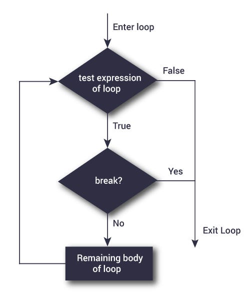
# Break statement is used to stop the loop in its tracks

for val in "Ahsan":
    if val == "n":
        break
    print(val)

print("loop end")

# Execute

A
h
s
a
loop end

Continue statement

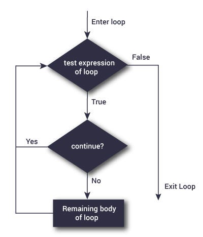
# Continue statement unlike break continues to print the statement till it finishes

for val in "Ahsan":
    if val == "a":
        continue
    print(val)

print("loop end")

# Execute

A
h
s
n
loop end

Good Python

Understanding Data Normalization

Deploying a neural network is an arduous process. One of the most important stages in developing a neural net is to first normalize the data. In this guide, I will explain why is normalization important, and finally how to normalize your data.

Problem: To predict if a person has children given the feature provided.

The input features (x-values, independent variables) need to be first normalized before we feed it to the neural network. In machine learning we call this process feature scaling or data preprocessing.

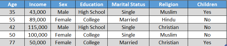
Given the example above we have the following features:

Input features (x-values or independent values): Age, Income, Sex, Education, Marital Status and Religion

Output feature (y-value or dependent value): Children

Question: Why is normalization important?

Answer: We have to normalize our data because our features do not have a uniform scale.

Most, if not all classifiers in machine learning calculate the Euclidean distance between the features. Euclidean distance is the “ordinary” straight-line distance between two points (vectors in a neural net) in Euclidean space.

Euclidean space is simply a 2 or 3 dimensional space. Hence, we normalize our features to remove any bias in our model. Also normalized data converges faster during backpropogation.

Question: How to normalize your data

**Answer: **In order to normalize your data, you will first need to learn the following methods:

Mix-max normalization

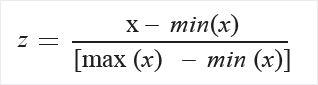
Take a value, subtract it by the minimum value and divide it by the difference of the maximum and minimum value. Normalizes the range of features to the range [0, 1] or [−1, 1].

2. Z-score normalization

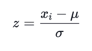
Take a value, subtract it by the mean of all values and divide it by the standard deviation of all the values. After normalization mean will be 0 and standard deviation will be 1.

3. Constant Normalization

Take your value and divide by a constant. Rule of thumb is to use constant values of a multiple of 10.

 = 55

= 10

 = 55/10 = 5.5

4. Binary Encoding

Categorical values like Gender can be encoded in either 0 or 1. Male can be encoded to 1, Female to 0.

Categorical values like Gender can also be encoded in either -1 or 1. Males can be encoded to -1, Female to 1.

5. Manhattan Encoding

If we have non-binary categorical data we can used Manhattan encoding which uses 0 or 1 o indicate if feature is included or excluded.

For e.g. In Religion class we can encode:

Muslim as a scalar of [ 1 0 0 ]

Hindu as a scalar [ 0 1 0 ]

Christian as a scalar [ 0 0 1 ]

Pro Tip: Use StandardScaler and OneHotEncoder for feature scaling in sci-kit learn library when coding

Understanding Gradient Descent and Backpropagation

A lot of data scientists use the term Gradient Descent and Backpropagation interchangeably, but contrary to popular opinion they are not the same thing.

What is Gradient Descent?

Gradient Descent is an optimization technique in the machine learning process which minimizes the cost function. Every machine learning algorithm has a cost function.

What is the Cost Function and why do I need to minimize it?

Whenever we use machine learning algorithms we are using the training data to make predictions which we later compare with the test data. The cost function is used to inform us how close are the real values from the training data to the predicted values in the test data. The closer the values, the lesser the accuracy error and the better our algorithm’s prediction prowess.

Gradient Descent is essentially an optimization algorithm we use in machine learning which helps us find the minimum point in the cost function (local minima or global minima). Think of gradient descent as a detective which is trying to find where the minimum point of the cost function. The minimum point of the cost function would mean the least amount of error.

If we map all the values of the cost function, we will see something like a 3D model akin to an undulating plane or mountain. Gradient descent is the method which is trying to find the lowest point in the 3D model. Again, the lowest point would mean for us the least error for our model. You can also picture gradient descent as a hiker trying to find the plateau on a hill. If the hiker finds the plateau he can’t go any lower. Similarly, if the gradient descent algorithm finds the minimum point, it will stop and wont go any further. We can then say that our model has converged.

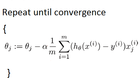
The alpha (learning rate) in the formula is how fast the algorithm converges. basically, we can control how slow or fast the hiker can go down the hill. If the learning rate is too small the hiker will very very slow and wont be able to reach the plateau. Similarly, if the learning rate is too large the hiker may walk past the plateau! The method by which the gradient descent algorithm works is by calculating derivatives which measures the rate of change of a slope.

What is Backpropagation?

In simple English, backpropagation is the method of computing the gradient of a cost function in deep neural nets. Unlike the gradient descent algorithm, backpropogation algorithm does not have a learning rate. Backpropagation instead finds the partial derivatives of the cost function.

In neural nets we have input layers for our input features, hidden layers to transform the inputs for our outputs and output layers for our desired outputs. Each neuron in the neural network has a corresponding weight and we change the weight to improve our performance. If by changing the weight we can improve the performance of the neural net we save that particular weight. To change one weight the neural net has to perform forward passes depending on the number of the hidden units, this is a slow and inefficient process. This is why we use backpropagation. Backpropagation allows us to compute the error derivatives of all hidden units at the same time.

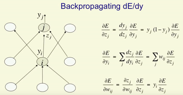
From the picture we can see that backpropagation works like forward pass but moves backwards from the hidden layer (i) to the input layer (j) and combines the error derivatives of all hidden layers at once. Backpropagation saves us time and helps us update the weights faster.

Conclusion

In a nutshell, the backpropagation algorithm computes how the error changes as we changes the weights in the neurons while the gradient descent algorithm optimizes the error of the cost function. In deep neural nets we use gradient descent and backpropagation in tandem to create the best models.

Back to blog

« Lstm Crime Predicition System »

Ahsan Anis